A Step by Step Backpropagation Example
(Backpropagation 예제를 활용한 한걸음)
Background (배경)
Backpropagation is a common method for training a neural network. There is no shortage of papers online that attempt to explain how backpropagation works, but few that include an example with actual numbers. This post is my attempt to explain how it works with a concrete example that folks can compare their own calculations to in order to ensure they understand backpropagation correctly.
If this kind of thing interests you, you should sign up for my newsletter where I post about AI-related projects that I’m working on.
(Backpropagation 은 뉴럴 네트워크 훈련에 일반적인 방법이다. 온라인상의 논문 부제로 backpropagation이 어떻게 작업을 하는지 실제 숫자를 포함하여 설명을 시도한다. )
Backpropagation in Python (파이썬에서 Backpropagation)
You can play around with a Python script that I wrote that implements the backpropagation algorithm in this Github repo.
(독자는 링크된 Github에서 구현된 backpropagation 알고리즘을 Python과 함께 실행할 수 있다.)
Backpropagation Visualization (Backpropagation 시각화)
For an interactive visualization showing a neural network as it learns, check out my Neural Network visualization.
(눈으로 볼수 있는 뉴런 네트워크는 학습은 "Neural Network Visualization"에서 확인해 보세요 )
Additional Resources (추가 자료)
If you find this tutorial useful and want to continue learning about neural networks and their applications, I highly recommend checking out Adrian Rosebrock’s excellent tutorial on Getting Started with Deep Learning and Python.
(독자들이 이 유용한 학습과 뉴런네트워크과 그 어플리케이션에 관심이 있으면, Adrian Rosebrock's의 훌륭한 가이드 "Getting Started with Deep Learning and Python"을 확인하기를 강력히 추천합니다.)
Overview (개요)
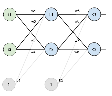
For this tutorial, we’re going to use a neural network with two inputs, two hidden neurons, two output neurons. Additionally, the hidden and output neurons will include a bias.
Here’s the basic structure:
(우리는 뉴런네트워크에 두개의 입력, 두개의 히든 뉴런, 두개의 출력을 사용한다. 추가적으로, 히든과 출력 뉴런은 바이어스를 포함한다. 여기는 기본 구조이다.
여기는 Backpropagation의 기본 구조이다.)
In order to have some numbers to work with, here are the initial weights, the biases, and training inputs/outputs:
(실제 숫자를 사용한 예제를 보이기 위해서 여러개의 초기 가중치, 여러개의 바이어스, 입력과 출력의 초기 값들을 아래와 같이 사용하였다.)
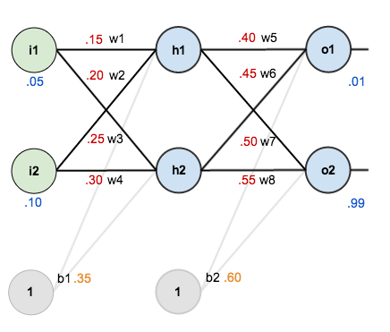
The goal of backpropagation is to optimize the weights so that the neural network can learn how to correctly map arbitrary inputs to outputs.
For the rest of this tutorial we’re going to work with a single training set: given inputs 0.05 and 0.10, we want the neural network to output 0.01 and 0.99.
(backpropabation의 목적은 가중치들을 최적화 하는것이다. 따라서 뉴런 네트워크는 임의 입력들에서 출력으로 정확한 맵을 학습할 수 있다. 아래의 학습을 설명하기 위해서 단일 훈련셋을 사용하였다. 주어진 입력은 0.05와 0.10, 출력은 0.01과 0.99이다.)
The Forward Pass (순 방향)
To begin, lets see what the neural network currently predicts given the weights and biases above and inputs of 0.05 and 0.10. To do this we’ll feed those inputs forward though the network.
(뉴럴 네트워크의 0.05와 0.10의 입력들의 주어진 가중치들과 바이어스들의 예측을보자. 이러한 입력값들을 이 네트워크를 향해서 넣어준다.)
We figure out the total net input to each hidden layer neuron, squash the total net input using an activation function (here we use the logistic function), then repeat the process with the output layer neurons.
(우리는 각각의 히든 레이어 뉴런에대한 전체 입력넷은 위와같다. 활성화 함수(여기서는 로직 함수를 사용)를 사용한 전체 입력망을 밀어 넣고, 다음으로 출력레이어 뉴런의 과정을 반반한다. )
Total net input is also referred to as just net input by some sources.
Here’s how we calculate the total net input for  :
:


(전체 입력넷<>을 다음과 같이 계산했다.
<h1의 입력은 각각 i1, i2와 b1과 연결되어있음을 그림에서 볼수 있고,
수식과 각각의 숫자를 대입하면 다음과 같다.> )
We then squash it using the logistic function to get the output of  :
:

( h1의 출력을 얻기위해서 로직함수를 사용하여 결과를 얻는다.)
Carrying out the same process for  we get:

(같은 절차대로 h2 결과를 얻는다.)
We repeat this process for the output layer neurons, using the output from the hidden layer neurons as inputs.
Here’s the output for  :
:


(히든 레이어 뉴런들로부터 결과를 사용하여, 출력 레이어 뉴런들에 위의 과정을 반복하였다<입력 레이어에서 했던것과 같이>.)
And carrying out the same process for  we get:

( 같은 절차대로 하여 02를 얻었다. )
Calculating the Total Error (전체 오차 계산)
We can now calculate the error for each output neuron using the squared error function and sum them to get the total error:
^{2}")
(전체 에러를 구하기 위해서 제곱 에러 함수와 그 합을 이용하여 각각의 아웃 뉴런의 에러를 계산한다.)
Some sources refer to the target as the ideal and the output as the actual.
The  is included so that exponent is cancelled when we differentiate later on. The result is eventually multiplied by a learning rate anyway so it doesn’t matter that we introduce a constant here [1].
For example, the target output for  is 0.01 but the neural network output 0.75136507, therefore its error is:
^{2} = \frac{1}{2}(0.01 - 0.75136507)^{2} = 0.274811083")
(예를 들어, o1에 대한 타겟 출력이 0.01 그러나 뉴럴 네트워크의 출력은 0.75136503, 그러므로 그 에러는 수식과 같다)
Repeating this process for  (remembering that the target is 0.99) we get:

(o2에대하여 똑같이 적용하면 (o2의 타겟은 0.99를 상기하며) 우리는 0.023560026를 얻는다)
The total error for the neural network is the sum of these errors:

(뉴럴 네트워크에대한 출력의 전체 에러는 이 에러들의 합이다.)
The Backwards Pass (역방향)
Our goal with backpropagation is to update each of the weights in the network so that they cause the actual output to be closer the target output, thereby minimizing the error for each output neuron and the network as a whole.
(backpropagation과 우리의 목적은 네트워크들의 가중치들을 각각 업데이트 시키는 것이다. 따라서 그 실체 출력은 타겟 출력에 더 가깝게 된다. 각각의 출력 뉴런과 네트워크의 에대한 에러가 최소화된다.)
Output Layer (출력 레이어)
Consider  . We want to know how much a change in
  affects the total error, aka
  .
.
(w5를 고려하자. w5의 변화가 전체 에러에 영항을 주는지 알고 싶다.)
 is read as “the partial derivative of
  with respect to
  “. You can also say “the gradient with respect to
  “.
“.
By applying the chain rule we know that:

( 체인 룰을 적용하여 우리는 알수 있다.)
Visually, here’s what we’re doing:
(시각화하면 아래와 같다)

We need to figure out each piece in this equation.
First, how much does the total error change with respect to the output?
^{2} + \frac{1}{2}(target_{o2} - out_{o2})^{2}")
^{2 - 1} * -1 + 0")
^{2 - 1} * -1 + 0")
 = -(0.01 - 0.75136507) = 0.74136507")
(이 방정식의 각 일부는 출력이 필요하다)
") is sometimes expressed as
is sometimes expressed as 
When we take the partial derivative of the total error with respect to  , the quantity
 ^{2}") becomes zero because
becomes zero because  does not affect it which means we’re taking the derivative of a constant which is zero.
Next, how much does the output of  change with respect to its total net input?
The partial derivative of the logistic function is the output multiplied by 1 minus the output:

 = 0.75136507(1 - 0.75136507) = 0.186815602")
Finally, how much does the total net input of  change with respect to
  ?
?

} + 0 + 0 = out_{h1} = 0.593269992")
Putting it all together:


You’ll often see this calculation combined in the form of the delta rule:
 * out_{o1}(1 - out_{o1}) * out_{h1}")
Alternatively, we have  and
and  which can be written as
  , aka
, aka  (the Greek letter delta) aka the node delta. We can use this to rewrite the calculation above:

 * out_{o1}(1 - out_{o1})")
Therefore:

Some sources extract the negative sign from  so it would be written as:

To decrease the error, we then subtract this value from the current weight (optionally multiplied by some learning rate, eta, which we’ll set to 0.5):

Some sources use  (alpha) to represent the learning rate, others use
  (eta), and others even use
  (epsilon).
We can repeat this process to get the new weights  ,
,  , and
, and  :
:


We perform the actual updates in the neural network after we have the new weights leading into the hidden layer neurons (ie, we use the original weights, not the updated weights, when we continue the backpropagation algorithm below).
Hidden Layer (히든 레이어)
Next, we’ll continue the backwards pass by calculating new values for  ,
,  ,
,  , and
, and  .
.
Big picture, here’s what we need to figure out:

Visually:
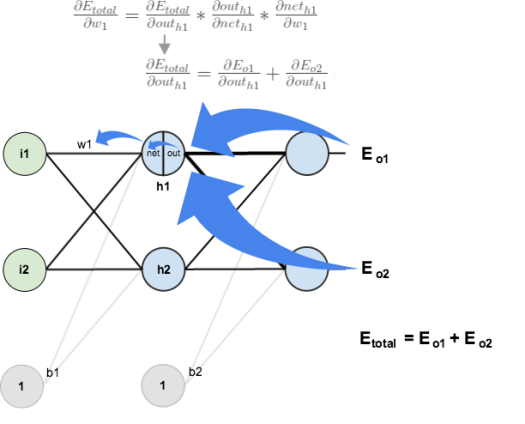
We’re going to use a similar process as we did for the output layer, but slightly different to account for the fact that the output of each hidden layer neuron contributes to the output (and therefore error) of multiple output neurons. We know that  affects both
  and
and  therefore the
  needs to take into consideration its effect on the both output neurons:

Starting with  :
:

We can calculate  using values we calculated earlier:

And  is equal to
  :
:


Plugging them in:

Following the same process for  , we get:

Therefore:

Now that we have  , we need to figure out
  and then
  for each weight:

 = 0.59326999(1 - 0.59326999 ) = 0.241300709")
We calculate the partial derivative of the total net input to  with respect to
  the same as we did for the output neuron:


Putting it all together:


You might also see this written as:
 * \frac{\partial out_{h1}}{\partial net_{h1}} * \frac{\partial net_{h1}}{\partial w_{1}}")
 * out_{h1}(1 - out_{h1}) * i_{1}")

We can now update  :
:

Repeating this for  ,
,  , and
, and 


Finally, we’ve updated all of our weights! When we fed forward the 0.05 and 0.1 inputs originally, the error on the network was 0.298371109. After this first round of backpropagation, the total error is now down to 0.291027924. It might not seem like much, but after repeating this process 10,000 times, for example, the error plummets to 0.000035085. At this point, when we feed forward 0.05 and 0.1, the two outputs neurons generate 0.015912196 (vs 0.01 target) and 0.984065734 (vs 0.99 target).
If you’ve made it this far and found any errors in any of the above or can think of any ways to make it clearer for future readers, don’t hesitate to drop me a note. Thanks!


